When you learn to make tables that are no longer limited to summing, differencing, quotienting and averaging, you can start to focus on how to multiply two or more cells. Cross product is something that you often use in mathematics. We can calculate the number of small points by heart, but the number is large, or plenty of number needs to be calculated, which is a little bit difficult at this point, so I think it is useful to choose to automatically compute the product in Excel, which can not only quick and accurate but also convenient.
So I’m going to share with you a little bit about how to do this in Excel. Whether you used to use Excel or not, I’m sure you’ll be able to take the product yourself after reading this tutorial.
2 methods to perform PRODUCT calculation on the data in Excel 2016
- Method 1: Type the formula to perform PRODUCT calculation
- Method 2: Insert function to perform PRODUCT calculation
Method 1: Type the formula to perform PRODUCT calculation
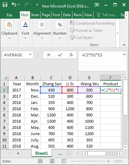
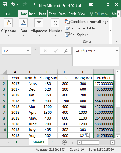
Step 1: Open the target Excel, type the formula “=C2*D2*E2” in the F2 cell and press Enter.
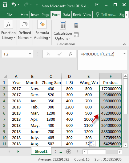
Or enter the formula “=PRODUCT(C2:D2:E2)” in the F2 cell and press Enter to display the product.

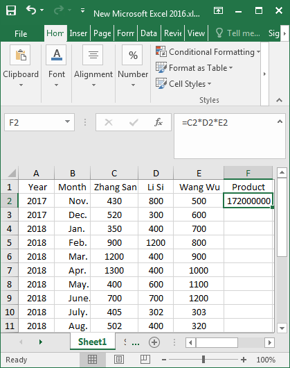
Step 2: As you can see, the product of C2:E2 displays in the F2 cell. Then move the cursor to the lower right corner of the F2 cell, press the left button of the mouse and drag it down when it is a solid black cross “+“.
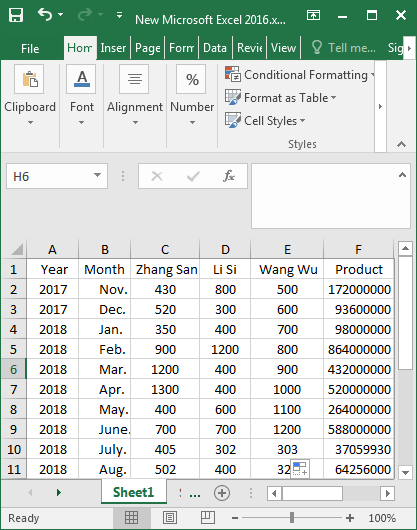
Step 3: When you let go of the mouse, you will find that all the calculations of the automatic cross-product are done, as shown in the figure below.
Method 2: Insert function to perform PRODUCT calculation
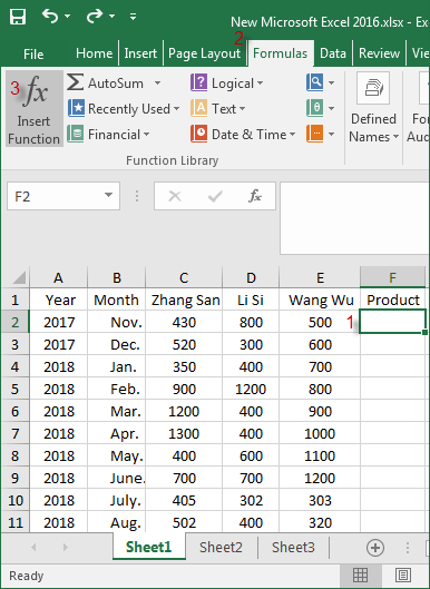
Step 1: Select the F2 cell, switch to the Formulas and click the Insert Function in the library group.
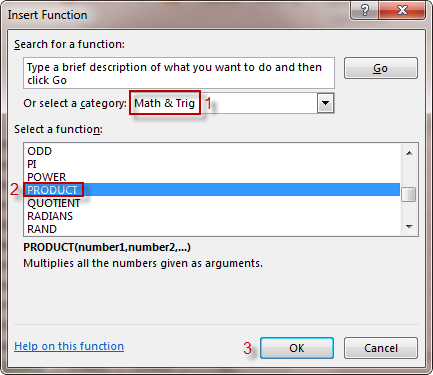
Step 2: The “Insert Function” dialog box pops up, select Math&Trig function in the category, then select PRODUCT function in the text box below, and click OK.
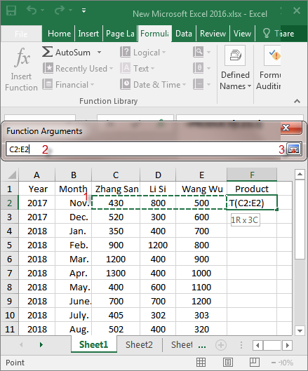
Step 3: The “Function Arguments” window will pop up, type C2:E2 in Number1, and click OK.
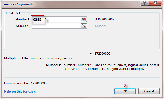
Alternatively, you can also choose to click the button with a red arrow.
![]()
This Function Arguments window will appear, select the region of C2:E2, and then C2:E2 will be displayed in the box. Click the red arrow button again.
Next, you’ll see C2:E2 in the Number1 box, and click OK.
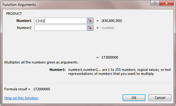
Step 4: At this time, the product of C2:E2 appears in F2 cell, and then move the cursor to the lower right corner of the F2 cell and drag down a solid black cross until all the automated cross-product calculations are displayed.