In the process of making tables, we may use Excel to perform various calculations on the data such as sum, difference, product, quotient, and average to complete our calculation. Calculating the average of all kinds of data is a very important parameter in the analysis data. If we use the traditional calculator to calculate the average, we need to repeatedly enter, and it is extremely easy to get the input data wrong during the input process.
However, calculating the average is one of the simplest and fastest methods in Excel, which can not only calculate the answer accurately but also check whether the data of each step is correct. Even in the face of massive data, we can easily calculate. Here’s how to calculate the average of the data in Excel 2016.
4 ways to calculate the average value of various data in Excel 2016
- Way 1: Insert function to calculate the average value
- Way 2: Using Average to calculate the average value
- Way 3: Enter the function formula to calculate the value
- Way 4: Enter the intricacy formula to calculate the value
Way 1: Insert function to calculate the average value
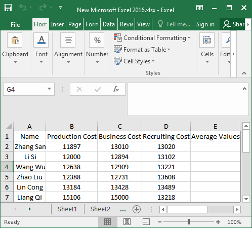
Step 1: Open the Excel table that requires to calculate the average value.
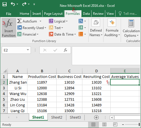
Step 2: Move the mouse into the first cell under the “Average Values“, then click the “Formulas” in the menu bar and select the “Insert Function” in the popular menu bar.
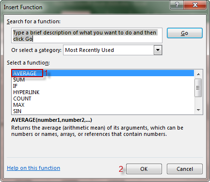
Step 3: When the Insert Function dialog box pops up, choose “AVERAGE” in the Select a function, you can see the detailed description of its function below, and then click OK.
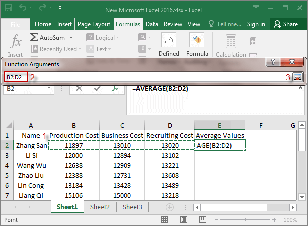
Step 4: In the Function Arguments window, click the red arrow button behind Number1. Click OK. Or just type B2:D2 behind Number1 and clickOK.
![]()
Step 5: Select the B2:D2 cell, and then B2:D2 will be displayed in the Function Arguments box. Click the red arrow button again.
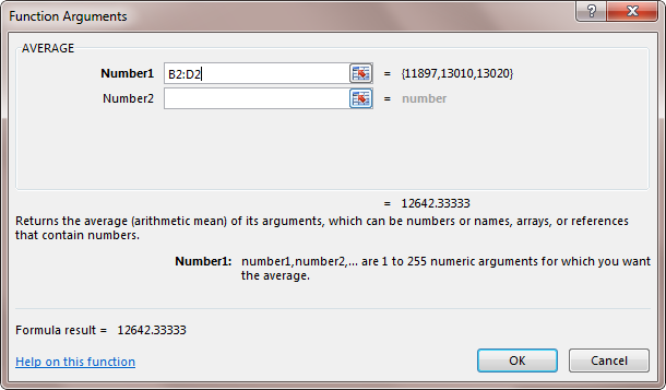
Step 6: You’ll see a dialog box with B2:D2 pops up and click OK.
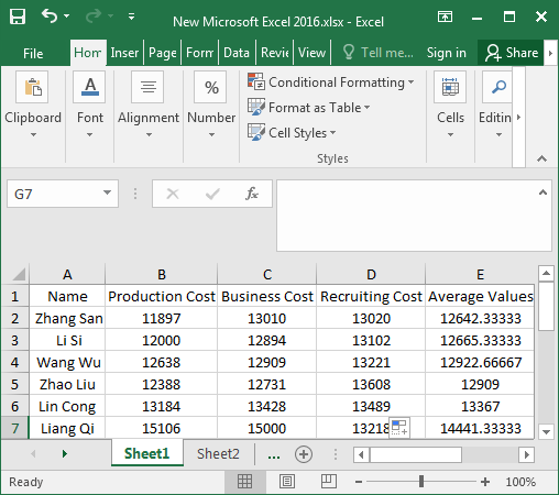
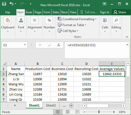
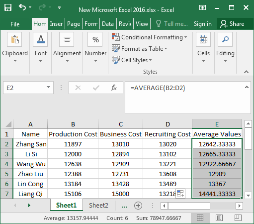
Step 7: At this point, the average of B2:D2 appears in the E2 cell.
Step 8: After calculating the average value of B2:D2, move the mouse into the lower right corner of the E2 cell, which will show the black “+” symbol. And just going to keep dragging it down until all of the data averages show up.
Way 2: Using Average to calculate the average value
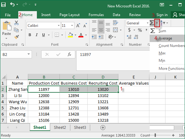
Step 1: Select the cell of B2:D2 and click the small arrow to select Average.
Step 2: Move the mouse into the lower right corner of the E2 cell, and a “+” symbol appears, drag it all the way down to E7.
Step 3: As you can see, the average value of column E has been calculated.
Way 3: Enter the function formula to calculate the average value
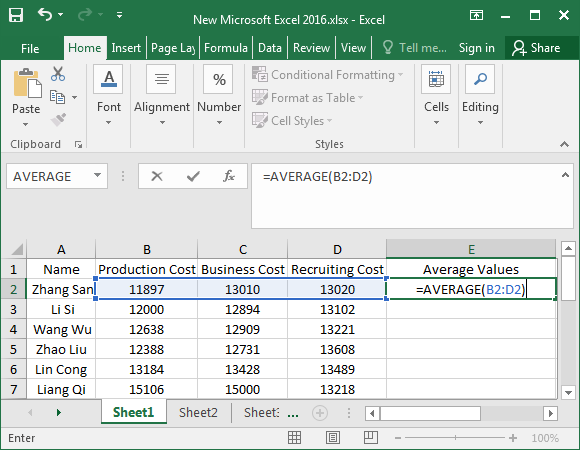
Enter the formula “=AVERAGE(B2:D2)” in the E2 cell and press “Enter” to display the average value. And go to Step 8 in way 1.
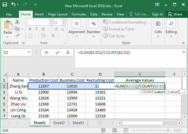
Way 4: Enter the intricacy formula to calculate the average value
Enter the formula “=SUM(B2:D2)/COUNT(B2:D2)” in the E2 cell, and press “Enter” to display the average value. And go to Step 8 in way 1.