In daily work, Excel table is a good helper for statistical data. Sometimes, we need to use an Excel table to make statistic data, such as making the statistics of student performance and company product price list or expense report. Thus, it is going to involve in summing, differencing, producting, and quotienting as well as averaging the data in the Excel table. In this article, we mainly introduce how to sum up the data in Excel 2016. Here are four different approaches provided for you.
- Way 1: Using AutoSum to sum up data
- Way 2: Enter the formula to sum up data
- Way 3: Insert function to sum up data
- Way 4: Press keyboards at one blow to sum up data
4 Ways to sum up the data in Excel 2016 table
If you store data such as price lists or reimbursement forms in Excel, you may need a quick way to sum up the price or amount. Today, I’ll show you how to easily sum up data in Excel 2016.
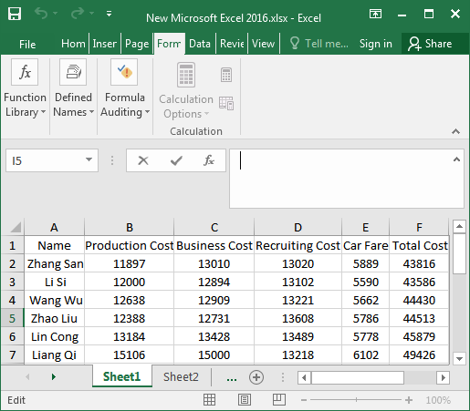
Way 1: Using AutoSum to sum up data
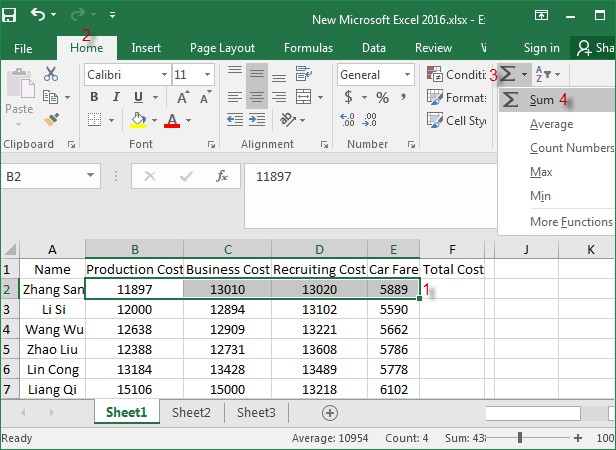
Step 1: Open the Excel table you want to sum up, select the first row of data, and then click the “AutoSum” button to choose Sum option in the upper right corner of the top toolbar.
Step 2: We will see that the result of the sum will appear in the cell at the end of the data area we selected. At this point, we select the cell with the result of the sum and move the mouse to the lower right corner of the cell until the mouse pointer changes to a solid cross shape. Once you see this solid cross shape appears, you pull down until it gets the summation data for all of this column.
Way 2: Enter the formula to sum up data
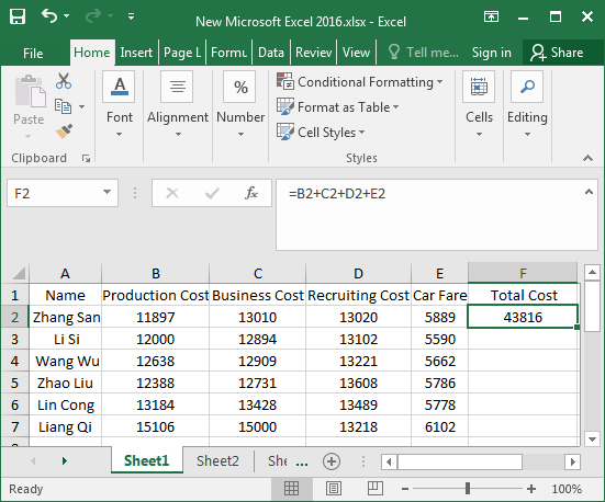
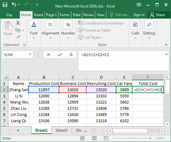
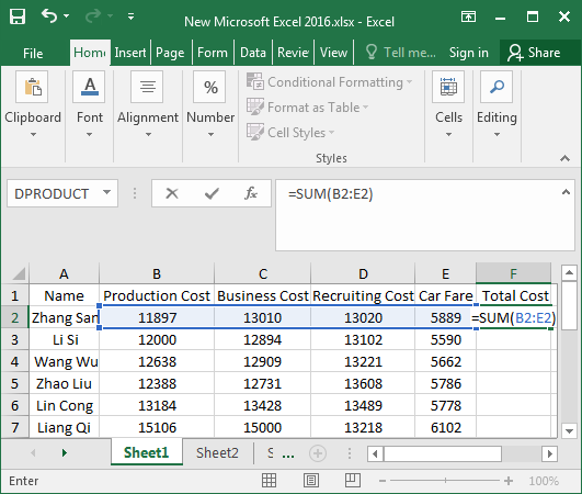
Step 1: Enter the formula: “=B2+C2+D2+E2” in the cell behind the data in the first row. After finishing the input, click any position of the extra edge of the cell.
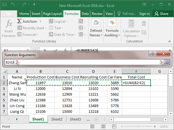
Or enter the formula “=SUM(B2:E2)” in the F2 cell and press “Enter” to display the sum.
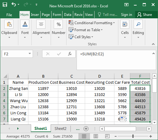
Step 2: Then we can use the previous method to drag the sign of the cross shape, and then all the data of the sum will be displayed.
Way 3: Insert function to sum up data
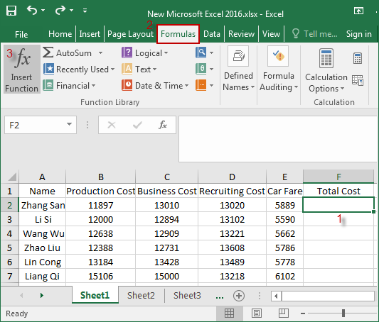
Step 1: Select the cell behind the data in the first row, and then select the Formulas > Insert Function.
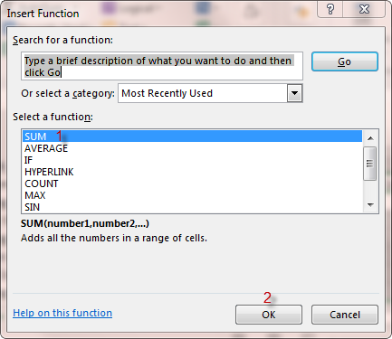
Step 2: In the Insert Function window. Select the SUM function and click OK.
Step 3: Type B2:E2 directly in the Number1 edit box, and then hit OK. At last, use the previous method to drag the sign of the cross shape, and then all the data of the sum will be displayed.
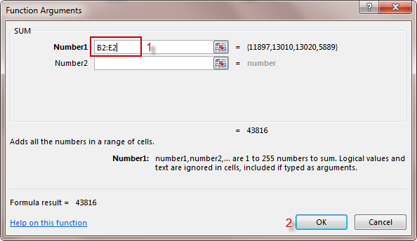
Alternatively, you can also choose to click the button with red arrows behind the edit box.
![]()
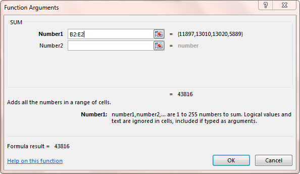
This Function Arguments window will appear, select the region to sum over, and then B2:E2 will be displayed in the window.
Next, you’ll see B2:E2 in the Number1 edit box (see the following figure), and finally click OK.
Way 4: Press keyboards at one blow to sum up data
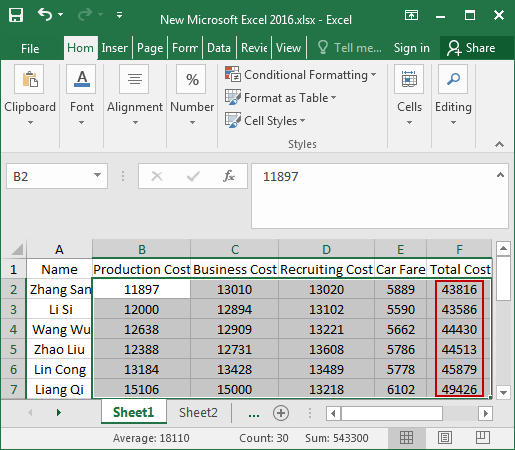
Step 1: Select all the data, as shown in the figure.
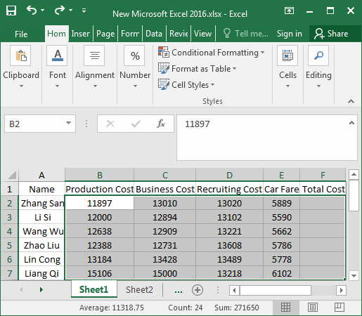
Step 2: Press “Alt and + =” keyboards simultaneously, and the data is all summed up.
The above are 4 ways of summing up the data in the Excel 2016 table. It’s a very simple operation. Have you learned them? Hopefully, this article will be of help to you!

