
When making an Excel worksheet, if you don’t want some of the data in the worksheet to be displayed, and you don’t want these important data looked up by the unapproved visitors. You can choose to completely hide the data in Excel 2016 worksheet. Here’s how to hide excel data completely for you!
Steps to completely hide the data in Excel 2016 worksheet
If you don’t want someone else to see something important in your Excel worksheet, you have to hide it.
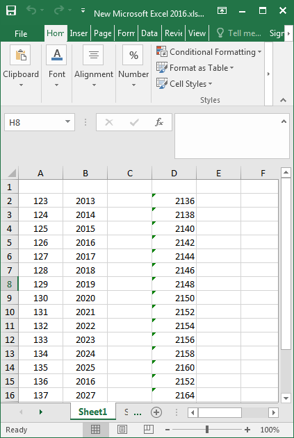
Step 1: Open the Excel worksheet with data.

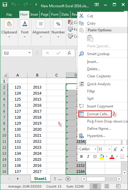
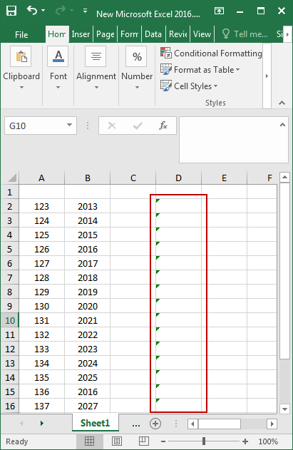
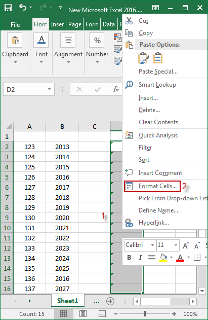
Step 2: Select cells with data that need to be hidden. For example, if you want to hide D row data, select it, then right-click to choose Format Cells.
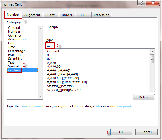
Step 3: A “Format Cells” dialog box pops up, choose Custom below the Number, and then enter three semicolons (;;;) in the box under Type on the right.

Step 4: Next, you can see that the data in the Excel worksheet is hidden.

Step 5: Right-click the cells again to select Format Cells.
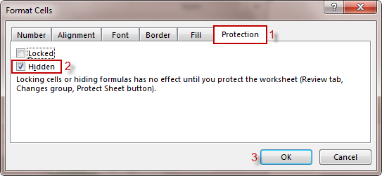
Step 6: Under Protection, select the Hidden option and press OK.

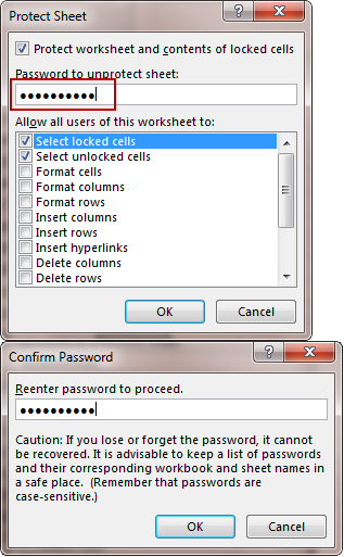
Step 7: Navigate to Review, select Protect Sheet.
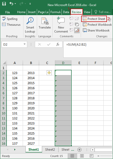

Step 8: When the “Protect Sheet” dialog box opens, set the password for protecting the Excel worksheet.

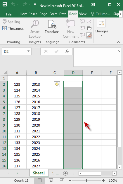
Step 9: After finished this setup, you can see that the data in the D row is completely gone.

The above is the method of completely hiding the Excel data, the operation is very simple, everybody can easily carry out according to the above operation steps, hoped this article can be helpful to everybody!