

Making charts with excel is part of the job. In order to make the charts more intuitive to reflect the data, many editors often create PivotTable in Excel 2016, but many friends are not clear about how to make the charts. Here is how to create PivotTable in Excel 2016.
Steps to create PivotTable in Excel 2016 manually
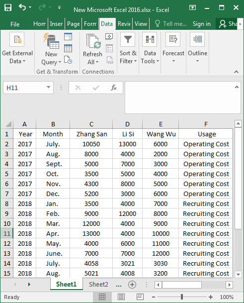
Step 1: Open the data document in excel 2016, which is the cost reimbursement situation of 3 salesmen in 2017-2018.

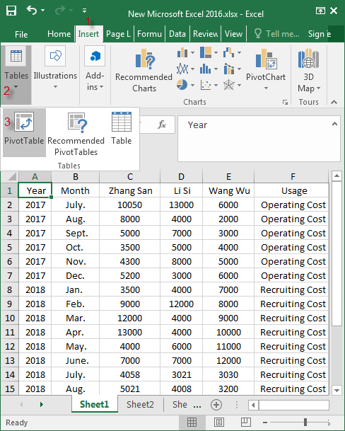
Step 2: Click any cell in the data area with the mouse, and click Insert, go to Tables > PivotTable.

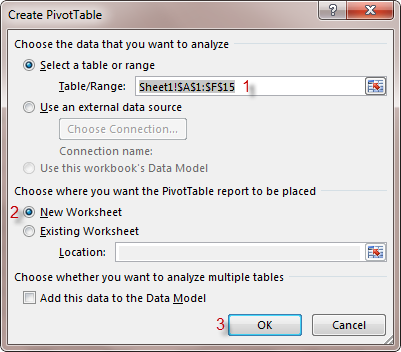
Step 3: At this time, a dialog box “Create PivotTable” pops up. You can see the data (Sheet1!$A$1:$F$15) we selected is displayed in the text behind “Table/Range“, then select New Worksheet and click OK.

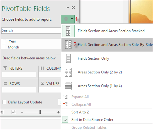
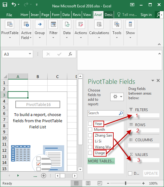
Step 4: In the PivotTable Fields list, click the triangle symbol on the right and select Fields Section and Areas Section Side-By-Side.

Step 5: Drag Year into FILTERS area, drag Usage into ROWS area and drag Zhang San, Li Si, Wang Wu into the VALUES area.

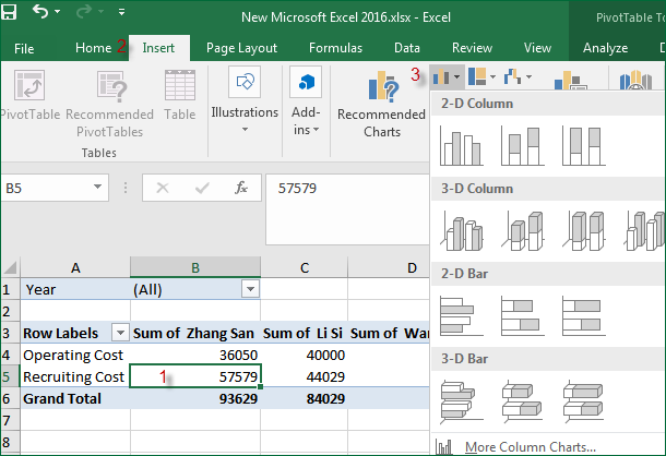
Step 6: After you select the options that need to be summarized, you can see that the table data will be summed up well. Click any cell that has aggregated the data, click Insert and choose the chart format you want.

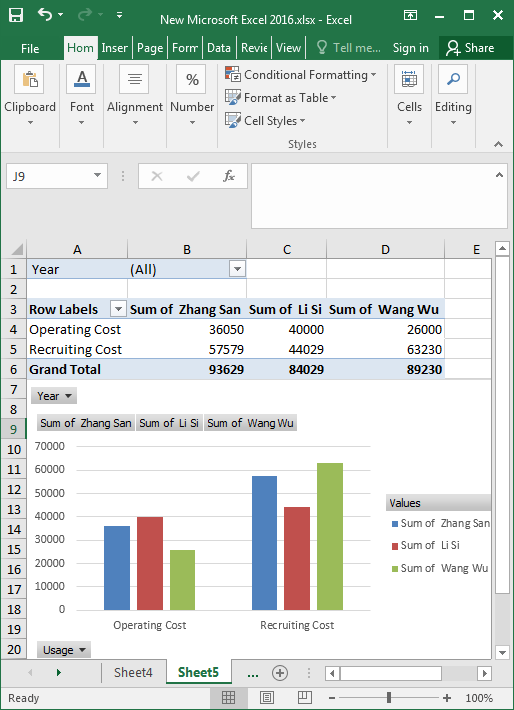
Step 7: Next, a PivotTable will be generated. Then you can see at a glance the sum of each person’s cost for operating and recruiting respectively.

The above is the method of creating the PivotTable in Excel 2016. The operation is so simple, you just follow the above steps to operate, I hope to help you!